Parallel Processing in Synapse Notebooks

Parallel processing refers to an operational process divided into parts and executed simultaneously across different compute resources to help optimize performance and decrease load times. This is especially important in processing many objects and large amounts of data. Azure Data Factory, Synapse Pipelines, and Fabric Pipelines provide out-of-the-box capabilities for parallel processing using the “ForEach” activity and deselecting the “Sequential” setting. There is also an optional “Batch count” setting that allows you to control the maximum number of parallel runs. If the Batch count setting is not set, it will try to execute as many parallel executions as possible using the Data Integration Units (DIU) allocated.

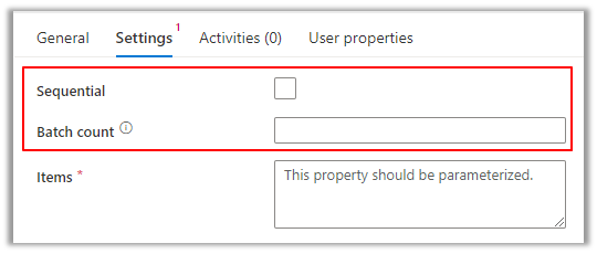
Image 1:  ForEach Activity parallel execution settings

You may be thinking, why not just parameterize a notebook and use it inside of a ForEach activity to iterate through the items you pass in? This would allow you to leverage the ForEach activities parallelization parameters; however, it has the following limitations: 

1. You cannot control spark pool sessions.

a. Each time a notebook runs, it starts a session.  This can take between 3 to 4 minutes in Synapse and ADF.  If you need to iterate through tens, hundreds, or even thousands of items, you can run into long wait times for new sessions to start.  

b. If other processes in the same data factory or Synapse environment use the same spark pool, you could run into timeouts or errors associated with limited resources. 

2. You are forced to use pipelines to call your notebooks.  While this is minor, and most architects and engineers will use a combination of pipelines and notebooks, it does require more costs as you are charged for pipeline and activity runs. 

Our architects and engineers in the Synapse workspace use a combination of pipelines and notebooks, so number two is not something that affects our team, but it is worth noting. Now that we understand the out-of-the-box capabilities and limitations—let’s cut to the use case and example to help optimize your notebook loads with parallel processing.

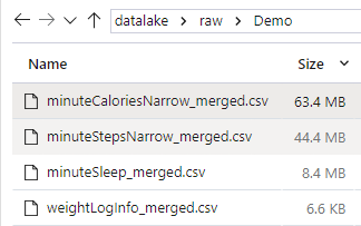
Image 2:  Four files in the raw data lake zone

The sizes are not huge- a couple are large enough to demonstrate the performance difference in serial versus parallel execution. 

We start with defining a few parameters to establish reusable values in later pieces of code: 

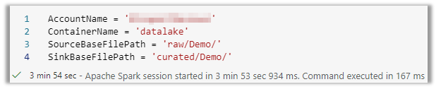
Image 3: Data lake connectivity and path parameters


As you can see, it took almost four minutes to start the spark session. However, once this session has started, any executions after this will be used in the same session.  To show execution times, we import a datetime library.

Image 4:  Datetime library

Next, we build the abfss endpoint to the data lake source location based on the parameters and then run the mssparkutils using that location to list all the files and write them to a data frame and collection. We will use this collection as the result set that we loop through and apply the load logic and parallelization code.

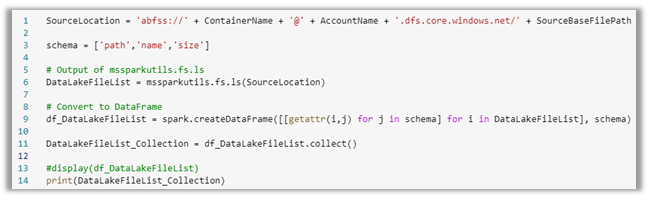
Image 5:  Build a collection of files in the source location

Image 6:  Collection of files and their properties

The below function, “parallel_load” contains code that will read the data of the raw data lake CSV file and write it to the curated data lake zone as a delta file. It will print out the file being processed when it started and when it finished. It is all wrapped in try/except logic to handle failures, if any.

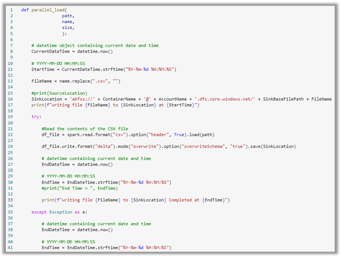
Image 7: load logic from raw to curated per file

You would execute the following code to execute this function in serial by passing one file at a time. This code takes each row in the collection and passes the values to the load function. As we can see below, it took 1 minute and 15 seconds to load all 4 files.

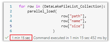
Image 8: load logic from raw to curated per file

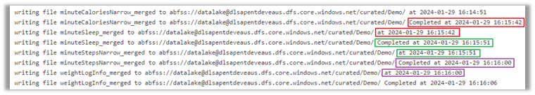
Image 9: Serial execution of each file shown by start and end times

Notice that only 1 file is run at a time in the result set, which is indicated by the start time of each file equal to the end time of the previous file.

Now, the fun part! Executing the load of these files in parallel requires threading and queueing Python libraries. Dustin Vannoy also has a blog and vlog on this. You can check it out here. I did not reinvent the wheel on this but used a different use case specific to data lake landing zones. I also wanted to shed light on comparisons between native parallelization in the ForEach activity in Pipelines versus Spark Pools and share some insights on errors I ran into. 

Parallel processing in Spark Notebooks requires threading and queue Python modules. The threading module is used to handle parallelization of tasks. The queue module is used along with the threading module to implement multi-producers between threads. We set a variable called WorkerCount, which is going to be how many files we want to run in parallel. This value can be modified to whatever you want, but remember that the spark pool size will determine how many resources it can handle.

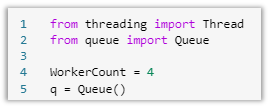
Image 10:  Threading and queue modules

We define a function “parallel_tasks” for retrieving items out of the queue using the get() class. Then, we unpack the collection of data values into individual items by using the *args variable. This function is wrapped into a try/except block to handle any failures unpacking the list of files. The “finally” block is very crucial. Once a file in the queue is unpacked and processed, you must call the task_done() class to mark the task as complete. This will prevent an infinite loop or reprocessing of already completed files.

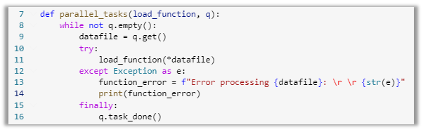
Image 11: Task function for looping through the queue

The next piece of code reads the data from the collection and places each row into the queue using the put() class.

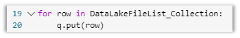
Image 12:  Putting each collection row into the queue

The last section of code runs a while loop to iterate through the list of files using the WorkerCount to determine how many items to run in parallel. The Thread() class accepts the queue of items unpacked by the “parallel_tasks” function and executes the load function “parallel_load.” We set the thread to a daemon, which runs in the background and is not expected to complete the operation before the entire program exits. This is all wrapped into a try/except block to handle any errors in the iterations within the function call. One of the most important pieces of this code is the join() class in the queue module. The join() class blocks until all items in the queue have been processed. This works in conjunction with the task_done() class.  Once an item in the queue is marked done, it drops out of the queue.  When all tasks are finished, the join() unblocks and ends.

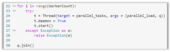
Image 13: Thread and queue assignment and iteration

Here is the script in its entirety:

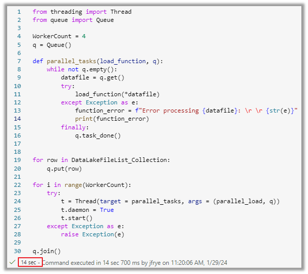
Image 14:  Entire script of threading and queueing files

As you can see from the command, it took 14 seconds to load all files in parallel from the raw lake to the curated lake as delta. This is exponentially faster than 1 minute and 15 seconds. That is a performance gain of over 80 percent! Below, you will see the printout of the results, showing all four files started at the same time based on the WorkerCount being set to 4.

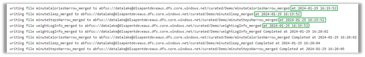
Image 15:  File start and end times for parallel executions

We have used a common, modern data integration scenario loading large amounts of data in parallel. You can leverage this for any type of processing scenario. It can also be translated to other platforms where pyspark/python code can be run.

Ready to innovate?

For businesses looking to empower their journey to cloud-scale analytics, Redapt offers a free tier of consulting through our Cloud-Scale Analytics Toolkit Offering.  

Or, to explore how your organization can leap into a new era of technological excellence and business growth, Contact Redapt today.